One of the less frequently used elements of the POV-Ray scene description language is the matrix keyword. Its primary functions are already handled by the easier-to-understand translate, scale and rotate keywords, and its non-intuitive syntax makes it a less-than-appealing area for new users to delve into.

      Yet it provides a simple mechanism by which objects can be skewed or slanted, which can be quite useful in certain tasks. Let us begin by examining the syntax of the keyword:

            matrix < 1, 0, 0,
                     0, 1, 0,
                     0, 0, 1,
                     0, 0, 0 >

      The matrix shown here is known as an identity matrix, which is to say, it leaves the object unchanged. The parameters in the above example have been colour-coded by function, to help show their relationships during the discussion below.

Scaling an object

      The boldface red characters (first, fifth and ninth in the array) control the object's scaling. The above example shows the equivalent of scaling the object by <1,1,1>. To scale an object by <2,3,4>, you would use the matrix:

            matrix < 2, 0, 0,
                     0, 3, 0,
                     0, 0, 4,
                     0, 0, 0 >

      As you can see, then, the first term controls the X scaling, the fifth term controls the Y scaling, and the ninth term controls the Z scaling.

Translating an object

      The bottom row, shown in blue italics, controls the translation of the object. The tenth through twelfth terms control the X translation, Y translation and Z translation respectively. To translate an object by <5,6,7>, you would use the matrix:

            matrix < 1, 0, 0,
                     0, 1, 0,
                     0, 0, 1,
                     5, 6, 7 >

      The two transformations can also be combined into one simple step. To produce both the scaling and translation shown in the previous two examples, you could use a single matrix transform:

            matrix < 2, 0, 0,
                     0, 3, 0,
                     0, 0, 4,
                     5, 6, 7 >

Skewing an object

      The remaining six terms control the skew of the object. As you can see, in each of the first three rows, there is one term which controls the scale along a particular axis, and two terms which control skew.

      Let us take as our example the first row. The first term controls the object's scaling along the X axis. The second term applies skew to the Y axis, and the third applies skew to the Z axis. But how is the skew calculated?

      The easiest way to explain is by demonstration. Let us create two boxes, and apply the following matrix transformation to one of them:

            matrix < 1.0, 0.5, 0.0,
                     0.0, 1.0, 0.0,
                     0.0, 0.0, 1.0,
                     0.0, 0.0, 0.0 >

      As you can see, the second box slants upwards as it moves along the X axis. Simply put, the position along the X axis is multiplied by the second term and added to the Y position. In this case, the second term is 0.5, so the amount added to the Y position is one half of the X position.

      Similarly, a value placed in the third term would be multiplied by the X position and added to the Z position. The same principle applies to the second and third rows; the fourth and sixth terms control the X and Z skew in relation to the object's position along the Y axis, and the seventh and eighth terms control the X and Y skew in relation to the Z position.

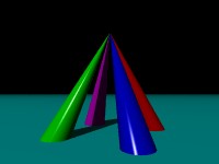
      Let us create four cones, slanting such that their tips touch in the middle, but their bases remain flat against the XZ plane. We'll create them with a bottom radius of 0.5, a height of 4, and place each of them two units from the origin along one of the X and Z axes.

      For the tips to meet, we'll need to apply a skew in the opposite direction of their positions along their respective axes; and since the slope will be two Y units for each X or Z unit, we'll use a multiplier of 0.5:

#include "colors.inc"

#declare Shiny = finish { phong 1.0 phong_size 100 }

cone { <2,0,0>, 0.5, <2,4,0>, 0
  matrix < 1.0, 0.0, 0.0,
          -0.5, 1.0, 0.0,
           0.0, 0.0, 1.0,
           0.0, 0.0, 0.0 >
  pigment { Red }  finish { Shiny }
}

cone { <-2,0,0>, 0.5, <-2,4,0>, 0
  matrix < 1.0, 0.0, 0.0,
           0.5, 1.0, 0.0,
           0.0, 0.0, 1.0,
           0.0, 0.0, 0.0 >
  pigment { Green }  finish { Shiny }
}

cone { <0,0,2>, 0.5, <0,4,2>, 0
  matrix < 1.0, 0.0, 0.0,
           0.0, 1.0,-0.5,
           0.0, 0.0, 1.0,
           0.0, 0.0, 0.0 >
  pigment { Magenta }  finish { Shiny }
}

cone { <0,0,-2>, 0.5, <0,4,-2>, 0
  matrix < 1.0, 0.0, 0.0,
           0.0, 1.0, 0.5,
           0.0, 0.0, 1.0,
           0.0, 0.0, 0.0 >
  pigment { Blue }  finish { Shiny }
}

plane { y, 0 pigment { Cyan }}
light_source { <-100,100,-100> colour 1 }

camera { location <-2.5,1.5,-6> look_at <0,2,0> }

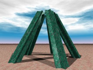
      As a more visually interesting example, let us now create a star-shaped column object, using an extruded prism, and then make five copies of it, skewing and translating each of them so that their tops touch at the points, and their bases slant out from the centre point.

#include "colors.inc"
#include "stones.inc"
#include "skies.inc"

#declare StarColumn = prism {
  linear_sweep linear_spline
  0, 10, 11,
  < 0.000, 1.000>, < 0.294, 0.405>, < 0.951, 0.309>, < 0.476,-0.155>,
  < 0.588,-0.809>, < 0.000,-0.500>, <-0.588,-0.809>, <-0.476,-0.155>,
  <-0.951, 0.309>, <-0.294, 0.405>, < 0.000, 1.000>
}

union {
  object { StarColumn 
    matrix < 1.000, 0.000, 0.000,
             0.000, 1.000,-0.500,
             0.000, 0.000, 1.000,
             0.000, 0.000, 6.500 >
  }
  object { StarColumn
    matrix < 1.000, 0.000, 0.000,
            -0.476, 1.000,-0.155,
             0.000, 0.000, 1.000,
             6.182, 0.000, 2.009 >
  }
  object { StarColumn
    matrix < 1.000, 0.000, 0.000,
            -0.294, 1.000, 0.405,
             0.000, 0.000, 1.000,
             3.821, 0.000,-5.259 >
  }
  object { StarColumn
    matrix < 1.000, 0.000, 0.000,
             0.294, 1.000, 0.405,
             0.000, 0.000, 1.000,
            -3.821, 0.000,-5.259 >
  }
  object { StarColumn
    matrix < 1.000, 0.000, 0.000,
             0.476, 1.000,-0.155,
             0.000, 0.000, 1.000,
            -6.182, 0.000, 2.009 >
  }
  texture { T_Stone18 }
}

plane { y, 0 texture { T_Stone5 }}
sky_sphere { S_Cloud2 }
light_source { <-100,200,-100> colour 1 }
light_source { <100,100,-50> colour 0.75 }

camera { location <5,3,-15> look_at <0,5,0> }

      Admittedly, we could have achieved similar (though not identical) results by simply rotating cones and star-shaped columns, then cutting off their ends by means of an intersection or difference. However, the ends thus produced would be distended; where the cone example above produces circular bases, a cone rotated to an angle and then cut off at the floor plane would have an oval base.

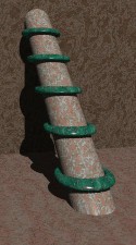
      Furthermore, consider the example of the image below: a cylinder with torus decorations, which has been skewed to an angle. The tori remain level, which would be difficult to achieve if the cylinder were merely rotated, because a plane cross-section of a rotated cylinder is not perfectly circular; the torus must either be distorted to match the cylinder's cross-section, or gaps between the cylinder and tori will become evident. By using the matrix keyword, however, the exercise becomes trivial.

      Unfortunately, the matrix syntax only permits linear transforms. It would be quite handy to have a skew based on a trigonometric function, for example, but this is not currently possible with POV-Ray.

Rotation:
Now it gets ugly.

      By combining the scaling and skew functions of the matrix, we can also rotate objects. This requires the use of the sine and cosine trigonometric functions. For instance, to rotate an object around the Z axis, we would use the following formula for a matrix transform:

x' = x * cos(a) - y * sin(a)
y' = x * sin(a) + y * cos(a)

      This formula is represented in the matrix syntax with the following construct:

            matrix < cos(a), sin(a), 0,
                    -sin(a), cos(a), 0,
                       0,      0,    1,
                       0,      0,    0 >

      If we were to rotate an object 45 degrees around the Z axis, we would use the following statement:

            matrix < 0.707, 0.707, 0.000,
                    -0.707, 0.707, 0.000,
                     0.000, 0.000, 1.000,
                     0.000, 0.000, 0.000 >

      Similar formulae are needed for rotations around the X and Y axes. Rotation may be combined with scaling and skewing, but this requires the use of matrix multiplication, which, given the ease of use of the rotate keyword, the author of this tutorial prefers to avoid.

      Other effects are possible, such as creating mirror images by specifying negative values for the scaling terms (this is also possible with the scale keyword), as the following code shows:

#include "colors.inc"

text { ttf "timesbd.ttf", "Test", 0.5, 0  pigment { Cyan }}

text { ttf "timesbd.ttf", "Test", 0.5, 0  pigment { Red }
  matrix < -1,0,0, 0,1,0, 0,0,1, 0,0,0 >
}

text { ttf "timesbd.ttf", "Test", 0.5, 0  pigment { Green }
  matrix < 1,0,0, 0,-1,0, 0,0,1, 0,0,0 >
}

text { ttf "timesbd.ttf", "Test", 0.5, 0  pigment { Blue }
  matrix < -1,0,0, 0,-1,0, 0,0,1, 0,0,0 >
}

camera { location <0,0,-3> look_at <0,0,0> }
light_source { <-100, 100,-200> colour rgb <1,1,1> }
light_source { < 100,-100,-200> colour rgb <1,1,1> }

      Although the rotate, translate and scale keywords are certainly much easier to use (and read) than their counterpart matrix constructs, the matrix keyword is still a useful component of the POV-Ray coder's toolbox.