The blob is an excellent way to create organic-looking shapes in POV-Ray, but it can be difficult to understand at first, because there are several variables which affect the physical shape of a blob. The most important are the threshold of the blob, the strength of each component, and the radius of each component.
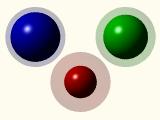
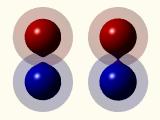
Observe the picture at the right, in which you can see three single-component blobs, each of which is surrounded by a mostly transparent sphere. Each blob consists of a spherical component with a radius of 1, which is the same radius of the surrounding sphere. Notice that the blob components appear to be smaller than their actual radius. This is due to the action of the threshold and strength keywords. The following table shows the interrelationship between all three components:
| actual radius | blob threshold | component strength | apparent radius | |
| Blue | 1.0 | 0.1 | 1.0 | 0.827 |
| Red | 1.0 | 0.5 | 1.0 | 0.541 |
| Green | 1.0 | 0.1 | 0.5 | 0.743 |
The density of each component is equal to the strength specified for that component at the exact centre, and equal to zero at the radius specified. The surface occurs when the density is exactly equal to the threshold specified for the entire blob.
The lower the threshold, the closer the apparent radius will be to the actual radius; the higher the threshold, the closer the apparent radius will be to the centre of the component. A higher threshold is better for connecting items smoothly to each other.
To determine what the apparent radius (a) of a component will be, you can use the formula:
a = sqrt( 1 - sqrt( threshold / strength )) * actual_radius
If you know what you want the apparent radius of a component to be, and you have already defined a threshold for the blob and an actual radius for the component, you can determine the proper component strength (s) with this formula:
s = threshold / ( 1 - ( apparent_radius / actual_radius )^2 )^2
These values are all interrelated. It is possible to create several apparently identical components by using different values for strength, threshold and the component radius, but the resulting components will react differently when multiple components are used within the blob.
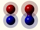
At left, you can see two different two-component blobs, with accompanying transparent spheres to show the actual radius of each component. Both blobs have a threshold of 0.4, and consist of two spherical components of radius 1, which are set a total of 1.5 units away from each other. The components of the left blob have a strength of 1.0, and the components of the right blob have a strength of 1.05.
The left blob's components are distended towards each other, where the radius of each component overlaps its neighbour. However, the field strength is not quite enough to merge the two components. A very small change (0.05) in the field strength was enough to merge them, as shown by the blob on the right.
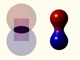
To widen the connecting bridge between the components without altering the apparent size of the spheres, it is necessary to increase the component radius while decreasing the component strength, as shown in the figure at the right.
It would also have been possible to alter the equation by changing the threshold value of the entire blob, but it is easier, when creating blobs with many components, to choose a single value for the threshold and leave it unchanged, altering only the component radius and strength to modify the components' appearance.
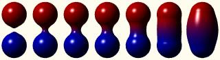
In general, the larger the actual radius of a component (assuming that its strength is modified to produce the same apparent radius), the "stickier" it becomes, which is to say, the thicker the "bridge" which is extruded to neighbouring components, as shown in the example below:
In the above image, the blobs are made from spherical components of radius 1.00, 1.05, 1.10, 1.125, 1.25, 1.50, and 1.75, respectively. The threshold value is 0.4 for all seven blobs, and the component strengths have been determined (using the second formula above) to provide the same apparent radius for the components.
Another way of connecting them would be to add a third, cylindrical component between the two. The image at left shows such a blob, along with the actual shapes and sizes of the components. Although this seems easier than calculating the values needed, as in the previous examples, it adds another layer of complexity to the equation, because the presence of the additional component can affect the apparent sizes of the others.
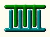
As a demonstration of this effect, observe the two comb-like structures constructed from cylindrical components, shown in the image at the right. The bottom structure's parts blend smoothly into each other, but the horizontal component in the top structure shows enlargements wherever a vertical component meets it.
This occurs because, in the top structure, the ends of the vertical components meet the centreline of the horizontal component. Because the components' field strengths are added together where they overlap, the apparent surface is pushed outwards at that point.
In the bottom structure, the vertical components extend only slightly into the actual radius of the horizontal one, and therefore the thickening only occurs in the area between the components.
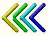
This principle also applies when joining the ends of cylindrical components. To the left, you can see four chevron-like structures. The leftmost (yellow) one is constructed of two cylinders which meet, and you can observe a bulbous thickening where their fields overlap.
In the second (green) chevron, each component stops just shy of meeting (in fact, the distance is equal to the components' actual radius). As you can see, the components still flow together, but there is a very obvious missing bit at the juncture between the two.
The third chevron (cyan) attempts to remedy this by placing a spherical component at the original joining point. Just to provide another example, however, the cylindrical components still meet at the same point occupied by the spherical one; notice how the bulbous region of overlap is even more pronounced than with the yellow example.
Finally, the rightmost (blue) chevron consists of a spherical component and two cylindrical components which end at the surface of the spherical component, producing a fairly smooth join amongst the three components.
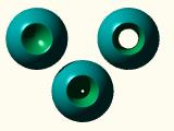
A component can be used to cut away parts of a blob, by specifying a negative strength. The field strength of the negative component is subtracted from the positive components. The example at right shows three spherical components, each of which has a strength of 1, and a cylindrical component subtracted from it using various negative strengths.
The upper-left sphere has a cylinder with strength -0.5 passing through it from front to back. As you can see, the cylinder looks more like a sphere which has been differenced out of the main component; this is because the cylinder's field strength is not enough to entirely negate the strength of the sphere.
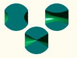
The bottom-centre sphere is modified by a cylinder with strength -1.0, the exact opposite of the sphere's strength. As can be seen by the cut-away views below, this appears as though the sphere is differenced by two cones set point-to-point.
The upper-right example shows a cylindrical component with a strength of -2.0 being used to cut away from the spherical component. This looks somewhat closer to the shape of a cylinder (though a much higher strength will be needed to keep the walls of the cylinder straight).
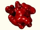
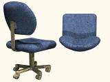
Once understood, the blob can easily be used to model both chaotic organic shapes, such as the red shape on the left, below, or regular shapes which are difficult to model with other constructive solid geometry primitives, such as the back cushion of the office chair shown in two views on the right.